Model Persamaan Struktural (SEM)
library(readxl)
#> Warning: package 'readxl' was built under R version 4.2.3
datasem <- read_excel("Data/Datalikert.xlsx")
head(datasem[,1:5])
#> # A tibble: 6 × 5
#>   Perusahaan Provinsi   Pulau    A1    A2
#>        <dbl> <chr>      <chr> <dbl> <dbl>
#> 1          1 Jawa Barat Jawa      4     5
#> 2          2 Jawa Timur Jawa      5     5
#> 3          3 Jawa Timur Jawa      4     4
#> 4          4 Jawa Barat Jawa      4     4
#> 5          5 Jawa Timur Jawa      4     4
#> 6          6 Jawa Timur Jawa      4     4
str(datasem)
#> tibble [300 × 45] (S3: tbl_df/tbl/data.frame)
#>  $ Perusahaan: num [1:300] 1 2 3 4 5 6 7 8 9 10 ...
#>  $ Provinsi  : chr [1:300] "Jawa Barat" "Jawa Timur" "Jawa Timur" "Jawa Barat" ...
#>  $ Pulau     : chr [1:300] "Jawa" "Jawa" "Jawa" "Jawa" ...
#>  $ A1        : num [1:300] 4 5 4 4 4 4 4 5 4 5 ...
#>  $ A2        : num [1:300] 5 5 4 4 4 4 4 5 4 5 ...
#>  $ A3        : num [1:300] 5 5 4 3 4 5 4 5 3 5 ...
#>  $ A4        : num [1:300] 4 5 4 4 3 4 4 5 3 5 ...
#>  $ A5        : num [1:300] 4 4 4 4 4 4 4 5 3 5 ...
#>  $ A6        : num [1:300] 4 5 4 4 4 4 4 5 3 4 ...
#>  $ A7        : num [1:300] 5 5 5 4 4 4 4 5 3 5 ...
#>  $ A8        : num [1:300] 5 5 5 4 4 4 4 5 3 4 ...
#>  $ Atotal    : num [1:300] 36 39 34 31 31 33 32 40 26 38 ...
#>  $ B1        : num [1:300] 4 4 4 4 3 5 3 3 3 4 ...
#>  $ B2        : num [1:300] 4 4 4 3 4 4 3 3 2 4 ...
#>  $ Btotal    : num [1:300] 8 8 8 7 7 9 6 6 5 8 ...
#>  $ C1        : num [1:300] 4 4 4 4 4 4 4 5 3 4 ...
#>  $ C2        : num [1:300] 4 4 4 4 4 4 4 4 3 4 ...
#>  $ Ctotal    : num [1:300] 8 8 8 8 8 8 8 9 6 8 ...
#>  $ D1        : num [1:300] 4 5 4 4 4 4 4 4 3 4 ...
#>  $ D2        : num [1:300] 4 5 4 3 4 5 4 4 2 4 ...
#>  $ D3        : num [1:300] 4 5 4 4 4 4 4 4 3 4 ...
#>  $ D4        : num [1:300] 4 5 4 5 4 4 4 4 3 4 ...
#>  $ Dtotal    : num [1:300] 16 20 16 16 16 17 16 16 11 16 ...
#>  $ E1        : num [1:300] 5 5 4 4 4 4 4 4 3 5 ...
#>  $ E2        : num [1:300] 5 5 4 4 4 5 4 4 3 5 ...
#>  $ E3        : num [1:300] 5 5 4 4 4 5 4 5 4 5 ...
#>  $ E4        : num [1:300] 4 5 4 3 4 5 4 4 3 4 ...
#>  $ E5        : num [1:300] 4 5 4 4 3 5 4 4 3 4 ...
#>  $ E6        : num [1:300] 4 5 4 4 4 4 4 4 3 4 ...
#>  $ E7        : num [1:300] 4 5 4 4 4 5 4 4 3 4 ...
#>  $ E8        : num [1:300] 4 5 4 4 3 5 4 4 3 4 ...
#>  $ E9        : num [1:300] 4 5 4 4 4 4 4 4 3 4 ...
#>  $ E10       : num [1:300] 4 5 4 4 4 5 4 5 3 4 ...
#>  $ E11       : num [1:300] 4 5 4 3 3 5 4 5 3 4 ...
#>  $ E12       : num [1:300] 5 5 4 4 4 5 4 5 3 5 ...
#>  $ Etotal    : num [1:300] 52 60 48 46 45 57 48 52 37 52 ...
#>  $ F1        : num [1:300] 5 5 4 4 4 5 4 4 2 4 ...
#>  $ F2        : num [1:300] 4 5 4 4 4 5 4 4 3 3 ...
#>  $ F3        : num [1:300] 4 5 4 4 4 4 4 4 2 3 ...
#>  $ F4        : num [1:300] 4 5 4 4 4 5 4 5 3 4 ...
#>  $ F5        : num [1:300] 4 5 4 4 3 5 4 4 3 3 ...
#>  $ F6        : num [1:300] 4 5 4 4 3 4 4 5 3 4 ...
#>  $ F7        : num [1:300] 4 5 4 4 3 4 4 4 3 4 ...
#>  $ F8        : num [1:300] 4 5 4 4 4 5 4 4 3 4 ...
#>  $ Ftotal    : num [1:300] 33 40 32 32 29 37 32 34 22 29 ...
attach(datasem)
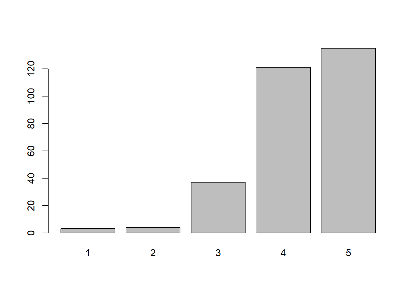
table(A1)
#> A1
#> 1 2 3 4 5
#> 3 4 37 121 135
# Spesifikasi Model
sem.model = "
faktor =~ A1 + A2 + A3 + A4
permintaan =~ B1 + B2
industri =~ C1 + C2
strategi =~ D1 + D2 + D3 + D4
regulasi =~ E1 + E2 + E3 + E4 + E5 + E6
kesempatan =~ F1 + F2 + F3 + F4
kesempatan ~ faktor + permintaan + industri + strategi + regulasi"
sem.fit = sem(sem.model, data = datasem)
summary(sem.fit, fit.measures=TRUE)
#> lavaan 0.6.17 ended normally after 90 iterations
#>
#>   Estimator                                         ML
#>   Optimization method                           NLMINB
#>   Number of model parameters                        59
#>
#>   Number of observations                           300
#>
#> Model Test User Model:
#>
#>   Test statistic                               555.757
#>   Degrees of freedom                               194
#>   P-value (Chi-square)                           0.000
#>
#> Model Test Baseline Model:
#>
#>   Test statistic                              7355.210
#>   Degrees of freedom                               231
#>   P-value                                        0.000
#>
#> User Model versus Baseline Model:
#>
#>   Comparative Fit Index (CFI)                    0.949
#>   Tucker-Lewis Index (TLI)                       0.940
#>
#> Loglikelihood and Information Criteria:
#>
#>   Loglikelihood user model (H0)              -4608.159
#>   Loglikelihood unrestricted model (H1)      -4330.280
#>
#>   Akaike (AIC)                                9334.318
#>   Bayesian (BIC)                              9552.841
#>   Sample-size adjusted Bayesian (SABIC)       9365.728
#>
#> Root Mean Square Error of Approximation:
#>
#>   RMSEA                                          0.079
#>   90 Percent confidence interval - lower         0.071
#>   90 Percent confidence interval - upper         0.087
#>   P-value H_0: RMSEA <= 0.050                    0.000
#>   P-value H_0: RMSEA >= 0.080                    0.410
#>
#> Standardized Root Mean Square Residual:
#>
#>   SRMR                                           0.035
#>
#> Parameter Estimates:
#>
#>   Standard errors                             Standard
#>   Information                                 Expected
#>   Information saturated (h1) model          Structured
#>
#> Latent Variables:
#>                    Estimate  Std.Err  z-value  P(>|z|)
#>   faktor =~
#>     A1                1.000
#>     A2                1.266    0.089   14.271    0.000
#>     A3                1.312    0.094   13.991    0.000
#>     A4                1.261    0.091   13.913    0.000
#>   permintaan =~
#>     B1                1.000
#>     B2                1.020    0.063   16.072    0.000
#>   industri =~
#>     C1                1.000
#>     C2                1.035    0.044   23.446    0.000
#>   strategi =~
#>     D1                1.000
#>     D2                0.973    0.033   29.472    0.000
#>     D3                0.972    0.043   22.590    0.000
#>     D4                0.817    0.042   19.325    0.000
#>   regulasi =~
#>     E1                1.000
#>     E2                0.929    0.039   23.666    0.000
#>     E3                0.950    0.043   22.088    0.000
#>     E4                1.015    0.039   25.697    0.000
#>     E5                0.985    0.042   23.464    0.000
#>     E6                0.913    0.045   20.186    0.000
#>   kesempatan =~
#>     F1                1.000
#>     F2                1.006    0.038   26.712    0.000
#>     F3                1.033    0.042   24.672    0.000
#>     F4                0.943    0.046   20.414    0.000
#>
#> Regressions:
#>                    Estimate  Std.Err  z-value  P(>|z|)
#>   kesempatan ~
#>     faktor            0.016    0.111    0.146    0.884
#>     permintaan        0.042    0.059    0.705    0.481
#>     industri          0.129    0.133    0.976    0.329
#>     strategi          0.131    0.091    1.449    0.147
#>     regulasi          0.685    0.077    8.860    0.000
#>
#> Covariances:
#>                    Estimate  Std.Err  z-value  P(>|z|)
#>   faktor ~~
#>     permintaan        0.233    0.034    6.785    0.000
#>     industri          0.327    0.037    8.729    0.000
#>     strategi          0.292    0.035    8.242    0.000
#>     regulasi          0.343    0.039    8.730    0.000
#>   permintaan ~~
#>     industri          0.366    0.043    8.447    0.000
#>     strategi          0.391    0.045    8.713    0.000
#>     regulasi          0.332    0.043    7.797    0.000
#>   industri ~~
#>     strategi          0.437    0.043   10.274    0.000
#>     regulasi          0.416    0.043    9.764    0.000
#>   strategi ~~
#>     regulasi          0.405    0.042    9.580    0.000
#>
#> Variances:
#>                    Estimate  Std.Err  z-value  P(>|z|)
#>    .A1                0.323    0.029   11.229    0.000
#>    .A2                0.161    0.018    8.902    0.000
#>    .A3                0.205    0.022    9.430    0.000
#>    .A4                0.198    0.021    9.552    0.000
#>    .B1                0.269    0.032    8.457    0.000
#>    .B2                0.078    0.025    3.161    0.002
#>    .C1                0.122    0.014    8.515    0.000
#>    .C2                0.106    0.014    7.549    0.000
#>    .D1                0.093    0.011    8.749    0.000
#>    .D2                0.063    0.008    7.476    0.000
#>    .D3                0.182    0.017   10.625    0.000
#>    .D4                0.200    0.018   11.219    0.000
#>    .E1                0.145    0.014   10.563    0.000
#>    .E2                0.114    0.011   10.395    0.000
#>    .E3                0.156    0.014   10.845    0.000
#>    .E4                0.091    0.010    9.488    0.000
#>    .E5                0.133    0.013   10.462    0.000
#>    .E6                0.198    0.018   11.224    0.000
#>    .F1                0.139    0.014    9.697    0.000
#>    .F2                0.090    0.011    8.221    0.000
#>    .F3                0.140    0.015    9.540    0.000
#>    .F4                0.233    0.021   10.912    0.000
#>     faktor            0.321    0.047    6.841    0.000
#>     permintaan        0.525    0.065    8.048    0.000
#>     industri          0.480    0.049    9.751    0.000
#>     strategi          0.522    0.050   10.406    0.000
#>     regulasi          0.542    0.055    9.811    0.000
#>    .kesempatan        0.122    0.015    8.068    0.000
sem.fit = sem(sem.model, data = datasem, std.lv=TRUE)
summary(sem.fit, fit.measures=TRUE, standardized=TRUE)
#> lavaan 0.6.17 ended normally after 90 iterations
#>
#>   Estimator                                         ML
#>   Optimization method                           NLMINB
#>   Number of model parameters                        59
#>
#>   Number of observations                           300
#>
#> Model Test User Model:
#>
#>   Test statistic                               555.757
#>   Degrees of freedom                               194
#>   P-value (Chi-square)                           0.000
#>
#> Model Test Baseline Model:
#>
#>   Test statistic                              7355.210
#>   Degrees of freedom                               231
#>   P-value                                        0.000
#>
#> User Model versus Baseline Model:
#>
#>   Comparative Fit Index (CFI)                    0.949
#>   Tucker-Lewis Index (TLI)                       0.940
#>
#> Loglikelihood and Information Criteria:
#>
#>   Loglikelihood user model (H0)              -4608.159
#>   Loglikelihood unrestricted model (H1)      -4330.280
#>
#>   Akaike (AIC)                                9334.318
#>   Bayesian (BIC)                              9552.841
#>   Sample-size adjusted Bayesian (SABIC)       9365.728
#>
#> Root Mean Square Error of Approximation:
#>
#>   RMSEA                                          0.079
#>   90 Percent confidence interval - lower         0.071
#>   90 Percent confidence interval - upper         0.087
#>   P-value H_0: RMSEA <= 0.050                    0.000
#>   P-value H_0: RMSEA >= 0.080                    0.410
#>
#> Standardized Root Mean Square Residual:
#>
#>   SRMR                                           0.035
#>
#> Parameter Estimates:
#>
#>   Standard errors                             Standard
#>   Information                                 Expected
#>   Information saturated (h1) model          Structured
#>
#> Latent Variables:
#>                    Estimate  Std.Err  z-value  P(>|z|)
#>   faktor =~
#>     A1                0.566    0.041   13.681    0.000
#>     A2                0.717    0.038   18.699    0.000
#>     A3                0.743    0.041   18.064    0.000
#>     A4                0.714    0.040   17.894    0.000
#>   permintaan =~
#>     B1                0.725    0.045   16.097    0.000
#>     B2                0.739    0.038   19.509    0.000
#>   industri =~
#>     C1                0.692    0.036   19.503    0.000
#>     C2                0.717    0.036   20.132    0.000
#>   strategi =~
#>     D1                0.723    0.035   20.812    0.000
#>     D2                0.703    0.033   21.615    0.000
#>     D3                0.702    0.038   18.344    0.000
#>     D4                0.590    0.036   16.459    0.000
#>   regulasi =~
#>     E1                0.736    0.038   19.623    0.000
#>     E2                0.684    0.034   19.941    0.000
#>     E3                0.699    0.037   18.967    0.000
#>     E4                0.747    0.035   21.120    0.000
#>     E5                0.725    0.037   19.819    0.000
#>     E6                0.673    0.038   17.720    0.000
#>   kesempatan =~
#>     F1                0.350    0.022   16.135    0.000
#>     F2                0.352    0.021   16.722    0.000
#>     F3                0.361    0.022   16.227    0.000
#>     F4                0.330    0.022   14.833    0.000
#>    Std.lv  Std.all
#>
#>     0.566    0.706
#>     0.717    0.872
#>     0.743    0.854
#>     0.714    0.849
#>
#>     0.725    0.813
#>     0.739    0.935
#>
#>     0.692    0.893
#>     0.717    0.911
#>
#>     0.723    0.922
#>     0.703    0.941
#>     0.702    0.855
#>     0.590    0.797
#>
#>     0.736    0.888
#>     0.684    0.897
#>     0.699    0.870
#>     0.747    0.927
#>     0.725    0.894
#>     0.673    0.834
#>
#>     0.771    0.900
#>     0.776    0.933
#>     0.796    0.905
#>     0.727    0.833
#>
#> Regressions:
#>                    Estimate  Std.Err  z-value  P(>|z|)
#>   kesempatan ~
#>     faktor            0.026    0.180    0.146    0.884
#>     permintaan        0.086    0.123    0.705    0.481
#>     industri          0.256    0.263    0.973    0.331
#>     strategi          0.272    0.188    1.447    0.148
#>     regulasi          1.443    0.190    7.608    0.000
#>    Std.lv  Std.all
#>
#>     0.012    0.012
#>     0.039    0.039
#>     0.116    0.116
#>     0.123    0.123
#>     0.654    0.654
#>
#> Covariances:
#>                    Estimate  Std.Err  z-value  P(>|z|)
#>   faktor ~~
#>     permintaan        0.568    0.046   12.297    0.000
#>     industri          0.833    0.025   33.258    0.000
#>     strategi          0.715    0.033   21.548    0.000
#>     regulasi          0.822    0.023   35.175    0.000
#>   permintaan ~~
#>     industri          0.729    0.035   20.610    0.000
#>     strategi          0.746    0.032   23.194    0.000
#>     regulasi          0.623    0.041   15.291    0.000
#>   industri ~~
#>     strategi          0.874    0.020   44.744    0.000
#>     regulasi          0.816    0.024   33.446    0.000
#>   strategi ~~
#>     regulasi          0.762    0.027   27.976    0.000
#>    Std.lv  Std.all
#>
#>     0.568    0.568
#>     0.833    0.833
#>     0.715    0.715
#>     0.822    0.822
#>
#>     0.729    0.729
#>     0.746    0.746
#>     0.623    0.623
#>
#>     0.874    0.874
#>     0.816    0.816
#>
#>     0.762    0.762
#>
#> Variances:
#>                    Estimate  Std.Err  z-value  P(>|z|)
#>    .A1                0.323    0.029   11.229    0.000
#>    .A2                0.161    0.018    8.902    0.000
#>    .A3                0.205    0.022    9.430    0.000
#>    .A4                0.198    0.021    9.552    0.000
#>    .B1                0.269    0.032    8.457    0.000
#>    .B2                0.078    0.025    3.161    0.002
#>    .C1                0.122    0.014    8.515    0.000
#>    .C2                0.106    0.014    7.549    0.000
#>    .D1                0.093    0.011    8.749    0.000
#>    .D2                0.063    0.008    7.476    0.000
#>    .D3                0.182    0.017   10.625    0.000
#>    .D4                0.200    0.018   11.219    0.000
#>    .E1                0.145    0.014   10.563    0.000
#>    .E2                0.114    0.011   10.395    0.000
#>    .E3                0.156    0.014   10.845    0.000
#>    .E4                0.091    0.010    9.488    0.000
#>    .E5                0.133    0.013   10.462    0.000
#>    .E6                0.198    0.018   11.224    0.000
#>    .F1                0.139    0.014    9.697    0.000
#>    .F2                0.090    0.011    8.221    0.000
#>    .F3                0.140    0.015    9.540    0.000
#>    .F4                0.233    0.021   10.912    0.000
#>     faktor            1.000
#>     permintaan        1.000
#>     industri          1.000
#>     strategi          1.000
#>     regulasi          1.000
#>    .kesempatan        1.000
#>    Std.lv  Std.all
#>     0.323    0.502
#>     0.161    0.239
#>     0.205    0.271
#>     0.198    0.280
#>     0.269    0.339
#>     0.078    0.126
#>     0.122    0.203
#>     0.106    0.171
#>     0.093    0.151
#>     0.063    0.114
#>     0.182    0.270
#>     0.200    0.365
#>     0.145    0.211
#>     0.114    0.195
#>     0.156    0.242
#>     0.091    0.141
#>     0.133    0.201
#>     0.198    0.304
#>     0.139    0.190
#>     0.090    0.130
#>     0.140    0.181
#>     0.233    0.306
#>     1.000    1.000
#>     1.000    1.000
#>     1.000    1.000
#>     1.000    1.000
#>     1.000    1.000
#>     0.206    0.206
#sem.fit = sem(sem.model, data = datasem, std.lv=TRUE, orthogonal=TRUE)
#summary(sem.fit, fit.measures=TRUE, standardized=TRUE)
# Modification Indices
modificationIndices(sem.fit, minimum.value = 10)
#>            lhs op rhs     mi    epc sepc.lv sepc.all
#> 72      faktor =~  D3 10.792  0.143   0.143    0.174
#> 82      faktor =~  F3 14.022 -0.170  -0.170   -0.193
#> 99  permintaan =~  E6 13.919  0.142   0.142    0.176
#> 112   industri =~  D3 19.393  0.315   0.315    0.383
#> 134   strategi =~  E3 11.975 -0.144  -0.144   -0.179
#> 152   regulasi =~  D3 18.808  0.197   0.197    0.240
#> 157   regulasi =~  F4 13.142  0.272   0.272    0.312
#> 168 kesempatan =~  D3 22.896  0.100   0.220    0.268
#> 175 kesempatan =~  E6 25.214  0.153   0.337    0.418
#> 176         A1 ~~  A2 15.863  0.068   0.068    0.298
#> 270         B1 ~~  F4 14.265  0.063   0.063    0.253
#> 317         D1 ~~  D3 10.752 -0.035  -0.035   -0.272
#> 331         D2 ~~  E1 11.098  0.025   0.025    0.257
#> 347         D3 ~~  E6 12.029  0.042   0.042    0.223
#> 351         D3 ~~  F4 10.217 -0.043  -0.043   -0.208
#> 352         D4 ~~  E1 11.953 -0.038  -0.038   -0.223
#> 362         E1 ~~  E2 17.329  0.038   0.038    0.294
#> 363         E1 ~~  E3 10.360  0.033   0.033    0.220
#> 364         E1 ~~  E4 12.186 -0.031  -0.031   -0.266
#> 371         E2 ~~  E3 11.663  0.032   0.032    0.236
#> 373         E2 ~~  E5 10.449 -0.028  -0.028   -0.231
#> 381         E3 ~~  E6 11.439 -0.039  -0.039   -0.221
#> 386         E4 ~~  E5 25.380  0.043   0.043    0.388
#> 398         E6 ~~  F2 14.478 -0.037  -0.037   -0.275
#> 399         E6 ~~  F3 20.998  0.052   0.052    0.310
#> 405         F2 ~~  F4 24.019 -0.058  -0.058   -0.404
#> 406         F3 ~~  F4 14.294  0.050   0.050    0.279
#>     sepc.nox
#> 72     0.174
#> 82    -0.193
#> 99     0.176
#> 112    0.383
#> 134   -0.179
#> 152    0.240
#> 157    0.312
#> 168    0.268
#> 175    0.418
#> 176    0.298
#> 270    0.253
#> 317   -0.272
#> 331    0.257
#> 347    0.223
#> 351   -0.208
#> 352   -0.223
#> 362    0.294
#> 363    0.220
#> 364   -0.266
#> 371    0.236
#> 373   -0.231
#> 381   -0.221
#> 386    0.388
#> 398   -0.275
#> 399    0.310
#> 405   -0.404
#> 406    0.279
sem.model2 = "
faktor =~ A1 + A2 + A3 + A4
permintaan =~ B1 + B2
industri =~ C1 + C2
strategi =~ D1 + D2 + D3 + D4
regulasi =~ E1 + E2 + E3 + E4 + E5 + E6
kesempatan =~ F1 + F2 + F3 + F4
kesempatan ~ faktor + permintaan + industri + strategi + regulasi
A1  ~~  A2
"
sem.fit = sem(sem.model2, data = datasem, std.lv=TRUE)
summary(sem.fit, fit.measures=TRUE, standardized=TRUE)
#> lavaan 0.6.17 ended normally after 94 iterations
#>
#>   Estimator                                         ML
#>   Optimization method                           NLMINB
#>   Number of model parameters                        60
#>
#>   Number of observations                           300
#>
#> Model Test User Model:
#>
#>   Test statistic                               540.535
#>   Degrees of freedom                               193
#>   P-value (Chi-square)                           0.000
#>
#> Model Test Baseline Model:
#>
#>   Test statistic                              7355.210
#>   Degrees of freedom                               231
#>   P-value                                        0.000
#>
#> User Model versus Baseline Model:
#>
#>   Comparative Fit Index (CFI)                    0.951
#>   Tucker-Lewis Index (TLI)                       0.942
#>
#> Loglikelihood and Information Criteria:
#>
#>   Loglikelihood user model (H0)              -4600.548
#>   Loglikelihood unrestricted model (H1)      -4330.280
#>
#>   Akaike (AIC)                                9321.095
#>   Bayesian (BIC)                              9543.322
#>   Sample-size adjusted Bayesian (SABIC)       9353.038
#>
#> Root Mean Square Error of Approximation:
#>
#>   RMSEA                                          0.077
#>   90 Percent confidence interval - lower         0.070
#>   90 Percent confidence interval - upper         0.085
#>   P-value H_0: RMSEA <= 0.050                    0.000
#>   P-value H_0: RMSEA >= 0.080                    0.303
#>
#> Standardized Root Mean Square Residual:
#>
#>   SRMR                                           0.035
#>
#> Parameter Estimates:
#>
#>   Standard errors                             Standard
#>   Information                                 Expected
#>   Information saturated (h1) model          Structured
#>
#> Latent Variables:
#>                    Estimate  Std.Err  z-value  P(>|z|)
#>   faktor =~
#>     A1                0.539    0.043   12.660    0.000
#>     A2                0.702    0.039   18.009    0.000
#>     A3                0.752    0.041   18.363    0.000
#>     A4                0.720    0.040   18.060    0.000
#>   permintaan =~
#>     B1                0.724    0.045   16.093    0.000
#>     B2                0.739    0.038   19.507    0.000
#>   industri =~
#>     C1                0.692    0.036   19.469    0.000
#>     C2                0.717    0.036   20.171    0.000
#>   strategi =~
#>     D1                0.723    0.035   20.813    0.000
#>     D2                0.703    0.033   21.613    0.000
#>     D3                0.702    0.038   18.345    0.000
#>     D4                0.590    0.036   16.460    0.000
#>   regulasi =~
#>     E1                0.736    0.038   19.615    0.000
#>     E2                0.684    0.034   19.943    0.000
#>     E3                0.699    0.037   18.964    0.000
#>     E4                0.747    0.035   21.115    0.000
#>     E5                0.726    0.037   19.826    0.000
#>     E6                0.673    0.038   17.728    0.000
#>   kesempatan =~
#>     F1                0.350    0.022   16.137    0.000
#>     F2                0.352    0.021   16.726    0.000
#>     F3                0.361    0.022   16.232    0.000
#>     F4                0.330    0.022   14.836    0.000
#>    Std.lv  Std.all
#>
#>     0.539    0.672
#>     0.702    0.854
#>     0.752    0.864
#>     0.720    0.855
#>
#>     0.724    0.813
#>     0.739    0.935
#>
#>     0.692    0.892
#>     0.717    0.912
#>
#>     0.723    0.922
#>     0.703    0.941
#>     0.702    0.855
#>     0.590    0.797
#>
#>     0.736    0.888
#>     0.684    0.897
#>     0.699    0.870
#>     0.747    0.927
#>     0.726    0.894
#>     0.673    0.834
#>
#>     0.771    0.900
#>     0.776    0.933
#>     0.796    0.905
#>     0.727    0.833
#>
#> Regressions:
#>                    Estimate  Std.Err  z-value  P(>|z|)
#>   kesempatan ~
#>     faktor            0.031    0.186    0.167    0.867
#>     permintaan        0.087    0.122    0.709    0.478
#>     industri          0.253    0.267    0.947    0.344
#>     strategi          0.272    0.189    1.442    0.149
#>     regulasi          1.441    0.190    7.578    0.000
#>    Std.lv  Std.all
#>
#>     0.014    0.014
#>     0.039    0.039
#>     0.115    0.115
#>     0.123    0.123
#>     0.654    0.654
#>
#> Covariances:
#>                    Estimate  Std.Err  z-value  P(>|z|)
#>  .A1 ~~
#>    .A2                0.068    0.019    3.588    0.000
#>   faktor ~~
#>     permintaan        0.573    0.046   12.417    0.000
#>     industri          0.837    0.025   33.458    0.000
#>     strategi          0.716    0.033   21.421    0.000
#>     regulasi          0.824    0.024   34.919    0.000
#>   permintaan ~~
#>     industri          0.729    0.035   20.581    0.000
#>     strategi          0.746    0.032   23.189    0.000
#>     regulasi          0.623    0.041   15.292    0.000
#>   industri ~~
#>     strategi          0.874    0.020   44.757    0.000
#>     regulasi          0.816    0.024   33.429    0.000
#>   strategi ~~
#>     regulasi          0.762    0.027   27.982    0.000
#>    Std.lv  Std.all
#>
#>     0.068    0.269
#>
#>     0.573    0.573
#>     0.837    0.837
#>     0.716    0.716
#>     0.824    0.824
#>
#>     0.729    0.729
#>     0.746    0.746
#>     0.623    0.623
#>
#>     0.874    0.874
#>     0.816    0.816
#>
#>     0.762    0.762
#>
#> Variances:
#>                    Estimate  Std.Err  z-value  P(>|z|)
#>    .A1                0.353    0.032   11.133    0.000
#>    .A2                0.182    0.020    9.132    0.000
#>    .A3                0.192    0.022    8.905    0.000
#>    .A4                0.190    0.021    9.171    0.000
#>    .B1                0.270    0.032    8.454    0.000
#>    .B2                0.078    0.025    3.155    0.002
#>    .C1                0.123    0.014    8.573    0.000
#>    .C2                0.104    0.014    7.494    0.000
#>    .D1                0.093    0.011    8.748    0.000
#>    .D2                0.063    0.008    7.481    0.000
#>    .D3                0.182    0.017   10.624    0.000
#>    .D4                0.200    0.018   11.218    0.000
#>    .E1                0.145    0.014   10.565    0.000
#>    .E2                0.114    0.011   10.392    0.000
#>    .E3                0.157    0.014   10.844    0.000
#>    .E4                0.092    0.010    9.490    0.000
#>    .E5                0.132    0.013   10.456    0.000
#>    .E6                0.197    0.018   11.222    0.000
#>    .F1                0.140    0.014    9.700    0.000
#>    .F2                0.090    0.011    8.219    0.000
#>    .F3                0.140    0.015    9.538    0.000
#>    .F4                0.233    0.021   10.912    0.000
#>     faktor            1.000
#>     permintaan        1.000
#>     industri          1.000
#>     strategi          1.000
#>     regulasi          1.000
#>    .kesempatan        1.000
#>    Std.lv  Std.all
#>     0.353    0.549
#>     0.182    0.270
#>     0.192    0.253
#>     0.190    0.268
#>     0.270    0.339
#>     0.078    0.125
#>     0.123    0.205
#>     0.104    0.169
#>     0.093    0.151
#>     0.063    0.114
#>     0.182    0.270
#>     0.200    0.365
#>     0.145    0.211
#>     0.114    0.195
#>     0.157    0.242
#>     0.092    0.141
#>     0.132    0.201
#>     0.197    0.304
#>     0.140    0.190
#>     0.090    0.130
#>     0.140    0.181
#>     0.233    0.306
#>     1.000    1.000
#>     1.000    1.000
#>     1.000    1.000
#>     1.000    1.000
#>     1.000    1.000
#>     0.206    0.206
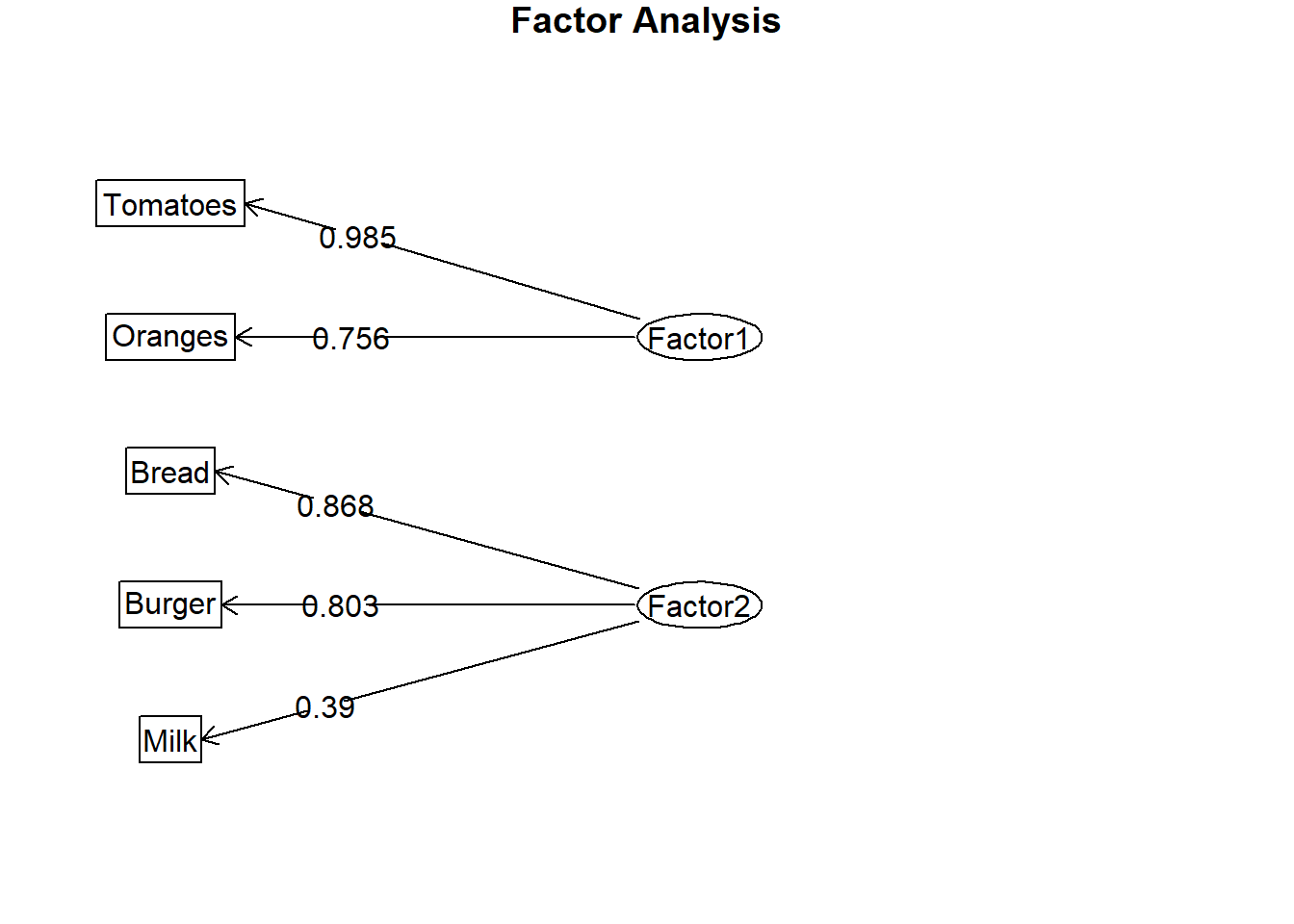
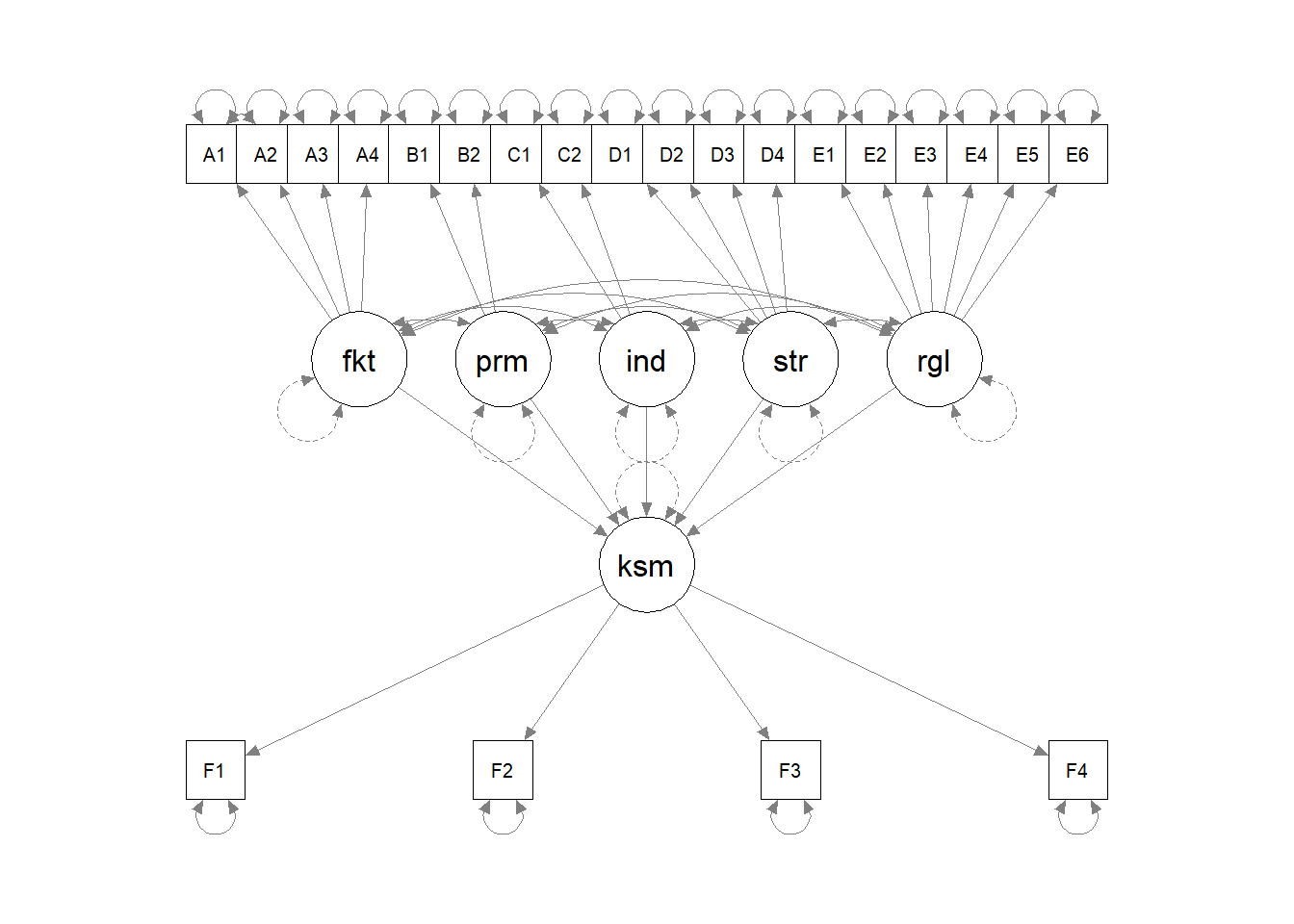
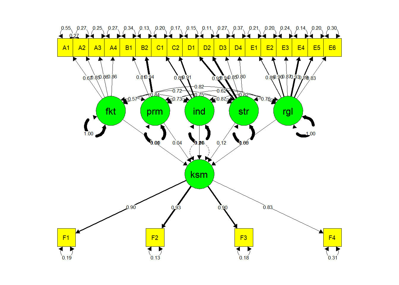
Visualisasi SEM
semPaths(sem.fit, "std",
         color = list(lat = "green", man = "yellow"),
         edge.color="black")
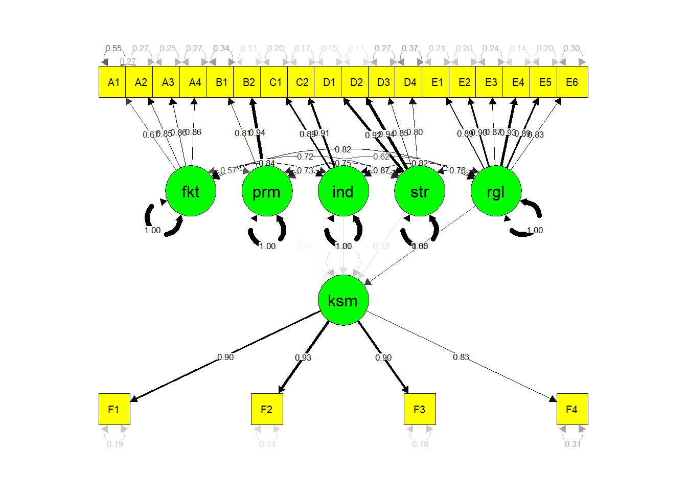
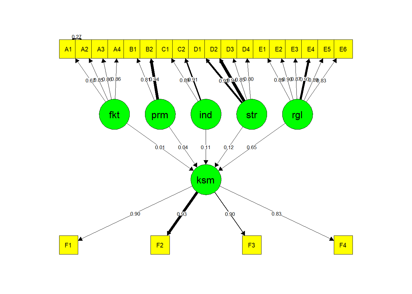
semPaths(sem.fit, "std",
         color = list(lat = "green", man = "yellow"),
         edge.color="black", fade=FALSE)
semPaths(sem.fit, "std",
         color = list(lat = "green", man = "yellow"),
         edge.color="black",
         fade=FALSE, residuals=FALSE, exoCov=FALSE)
PLS SEM
# source:https://rpubs.com/ifn1411/PLS
# install plspm
#install.packages("plspm")
# load plspm
library(plspm)
#> Warning: package 'plspm' was built under R version 4.2.3
#>
#> Attaching package: 'plspm'
#> The following objects are masked from 'package:psych':
#>
#>     alpha, rescale, unidim
# load data spainmodel
data(spainfoot)
# first 5 row of spainmodel data
head(spainfoot)
#>            GSH GSA  SSH  SSA GCH GCA  CSH  CSA WMH WMA LWR
#> Barcelona   61  44 0.95 0.95  14  21 0.47 0.32  14  13  10
#> RealMadrid  49  34 1.00 0.84  29  23 0.37 0.37  14  11  10
#> Sevilla     28  26 0.74 0.74  20  19 0.42 0.53  11  10   4
#> AtleMadrid  47  33 0.95 0.84  23  34 0.37 0.16  13   7   6
#> Villarreal  33  28 0.84 0.68  25  29 0.26 0.16  12   6   5
#> Valencia    47  21 1.00 0.68  26  28 0.26 0.26  12   6   5
#>            LRWL  YC RC
#> Barcelona    22  76  6
#> RealMadrid   18 115  9
#> Sevilla       7 100  8
#> AtleMadrid    9 116  5
#> Villarreal   11 102  5
#> Valencia      8 120  6
Attack <-  c(0, 0, 0)
Defense <- c(1, 0, 0)
Success <- c(1, 0, 0)

model_path <- rbind(Attack, Defense, Success)
colnames(model_path) <- rownames(model_path)

model_path
#>         Attack Defense Success
#> Attack       0       0       0
#> Defense      1       0       0
#> Success      1       0       0
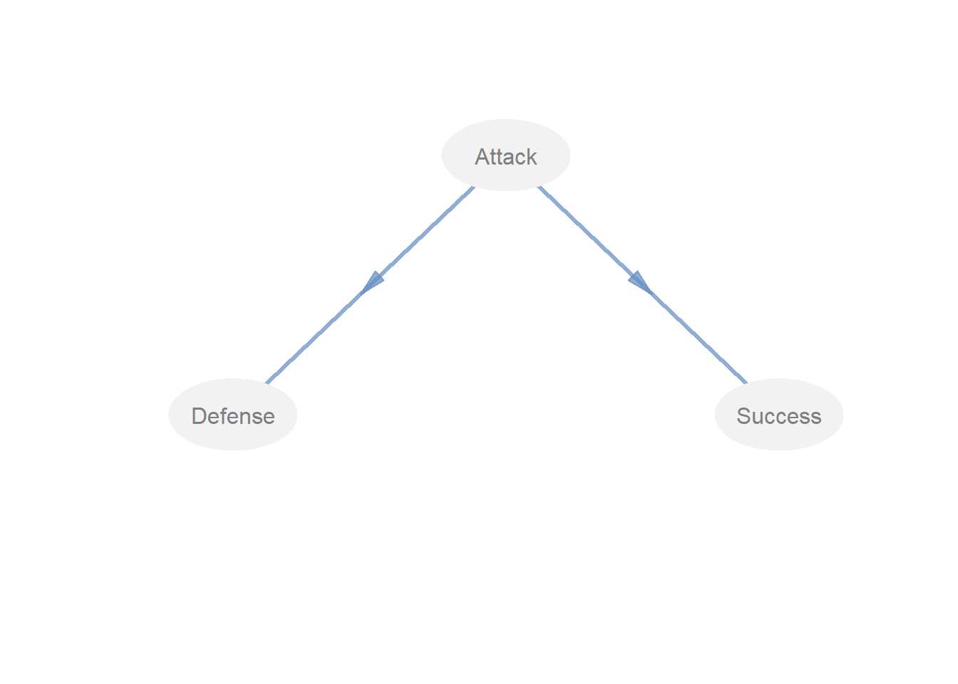
# graph structural model
innerplot(model_path)
Attack <-  c(0, 1, 0)
Defense <- c(0, 0, 0)
Success <- c(1, 1, 0)

model_path2 <- rbind(Attack, Defense, Success)
colnames(model_path2) <- rownames(model_path2)

model_path2
#>         Attack Defense Success
#> Attack       0       1       0
#> Defense      0       0       0
#> Success      1       1       0
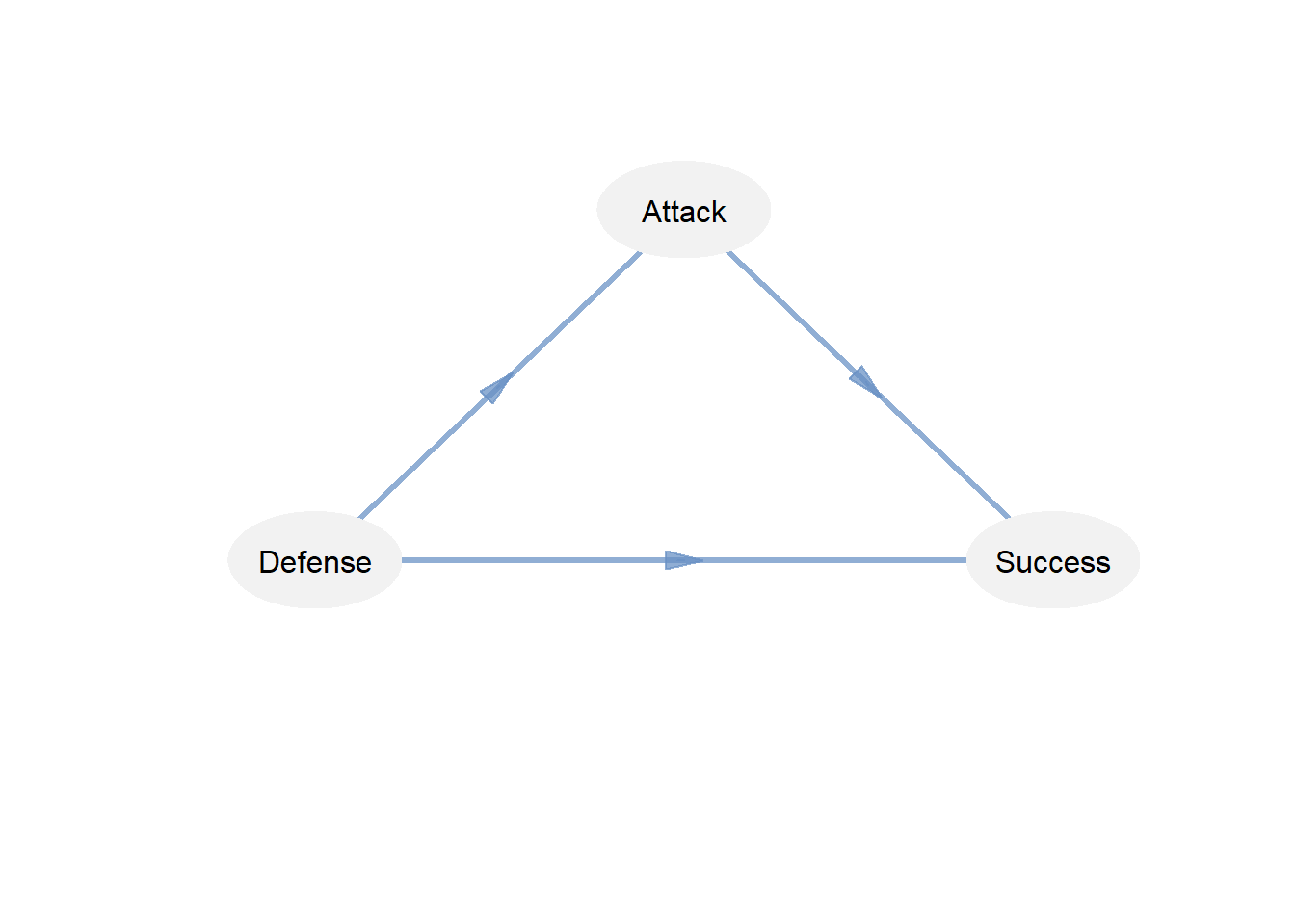
# graph structural model
innerplot(model_path2, txt.col = "black")
# define latent variable associated with
model_blocks <- list(1:4, 5:8, 9:12)

# vector of modes (reflective)
model_modes <- c("A", "A", "A")

# run plspm analysis
model_pls <- plspm(Data = spainfoot, path_matrix = model_path, blocks = model_blocks, modes = model_modes)

model_pls
#> Partial Least Squares Path Modeling (PLS-PM)
#> ---------------------------------------------
#>    NAME             DESCRIPTION
#> 1  $outer_model     outer model
#> 2  $inner_model     inner model
#> 3  $path_coefs      path coefficients matrix
#> 4  $scores          latent variable scores
#> 5  $crossloadings   cross-loadings
#> 6  $inner_summary   summary inner model
#> 7  $effects         total effects
#> 8  $unidim          unidimensionality
#> 9  $gof             goodness-of-fit
#> 10 $boot            bootstrap results
#> 11 $data            data matrix
#> ---------------------------------------------
#> You can also use the function 'summary'
# Unidimensionality
model_pls$unidim
#>         Mode MVs   C.alpha     DG.rho  eig.1st   eig.2nd
#> Attack     A   4 0.8905919 0.92456079 3.017160 0.7923055
#> Defense    A   4 0.0000000 0.02601677 2.393442 1.1752781
#> Success    A   4 0.9165491 0.94232868 3.217294 0.5370492
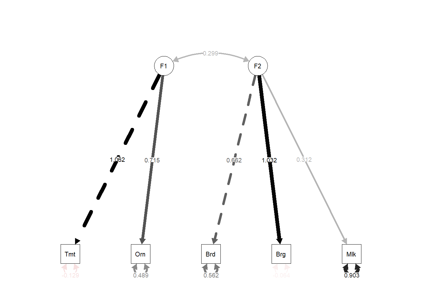
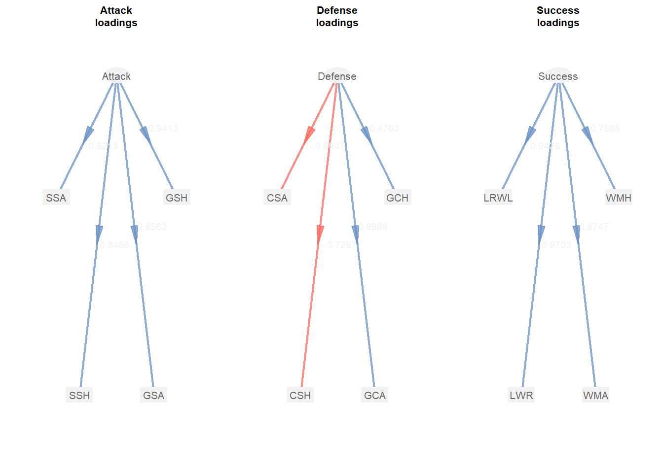
plot(model_pls, what = "loadings")
# Loadings and Communilaties
model_pls$outer_model
#>    name   block     weight    loading communality
#> 1   GSH  Attack  0.3474771  0.9412506   0.8859527
#> 2   GSA  Attack  0.2671782  0.8562398   0.7331465
#> 3   SSH  Attack  0.2922077  0.8466039   0.7167381
#> 4   SSA  Attack  0.2396012  0.8212987   0.6745316
#> 5   GCH Defense -0.1198790  0.4762965   0.2268583
#> 6   GCA Defense -0.4264164  0.8885714   0.7895590
#> 7   CSH Defense  0.2949470 -0.7297095   0.5324759
#> 8   CSA Defense  0.3898039 -0.8947452   0.8005689
#> 9   WMH Success  0.2484276  0.7884562   0.6216632
#> 10  WMA Success  0.2691511  0.8747163   0.7651285
#> 11  LWR Success  0.2947322  0.9703409   0.9415614
#> 12 LRWL Success  0.2998524  0.9428112   0.8888929
#>    redundancy
#> 1  0.00000000
#> 2  0.00000000
#> 3  0.00000000
#> 4  0.00000000
#> 5  0.05071506
#> 6  0.17650898
#> 7  0.11903706
#> 8  0.17897028
#> 9  0.49452090
#> 10 0.60864477
#> 11 0.74899365
#> 12 0.70709694
# Crossloadings
model_pls$crossloadings
#>    name   block     Attack    Defense    Success
#> 1   GSH  Attack  0.9412506 -0.5139001  0.9019257
#> 2   GSA  Attack  0.8562398 -0.3403294  0.7483558
#> 3   SSH  Attack  0.8466039 -0.4124617  0.7781795
#> 4   SSA  Attack  0.8212987 -0.3455460  0.6308989
#> 5   GCH Defense -0.1302683  0.4762965 -0.1620567
#> 6   GCA Defense -0.4633220  0.8885714 -0.5640722
#> 7   CSH Defense  0.3204993 -0.7297095  0.4850456
#> 8   CSA Defense  0.4235465 -0.8947452  0.5811253
#> 9   WMH Success  0.7126127 -0.4120502  0.7884562
#> 10  WMA Success  0.7720228 -0.7147787  0.8747163
#> 11  LWR Success  0.8454164 -0.5345709  0.9703409
#> 12 LRWL Success  0.8600973 -0.5910943  0.9428112
# Coefficient of Determination
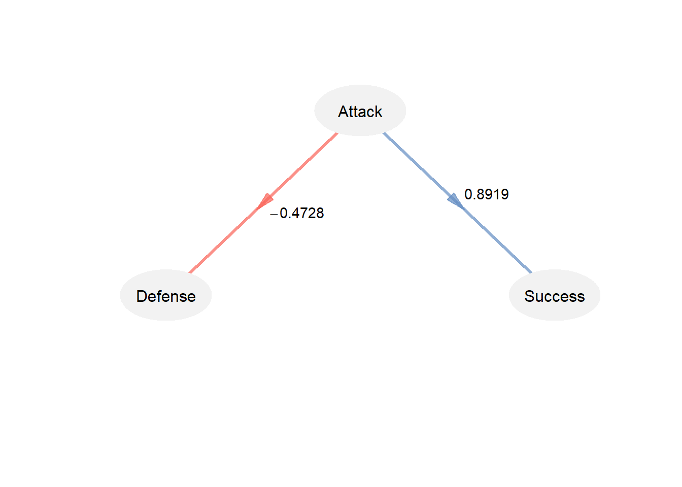
model_pls$inner_model
#> $Defense
#> Estimate Std. Error t value Pr(>|t|)
#> Intercept 5.504973e-17 0.2076918 2.650549e-16 1.00000000
#> Attack -4.728148e-01 0.2076918 -2.276521e+00 0.03526176
#>
#> $Success
#> Estimate Std. Error t value Pr(>|t|)
#> Intercept 7.783183e-17 0.1065936 7.301735e-16 1.000000e+00
#> Attack 8.918971e-01 0.1065936 8.367266e+00 1.285711e-07
# Redundancy
model_pls$inner_summary
#>               Type        R2 Block_Communality
#> Attack   Exogenous 0.0000000         0.7525922
#> Defense Endogenous 0.2235539         0.5873656
#> Success Endogenous 0.7954804         0.8043115
#>         Mean_Redundancy       AVE
#> Attack        0.0000000 0.7525922
#> Defense       0.1313078 0.5873656
#> Success       0.6398141 0.8043115
# Goodness-of-fit
model_pls$gof
#> [1] 0.6034738
plot(model_pls, what = "inner", colpos = "#6890c4BB", colneg = "#f9675dBB", txt.col = "black", arr.tcol="black")