1 Basics of R
1.1 Introduction
A <- 2
A # Print A
#> [1] 2
A = 2
A
#> [1] 2
B <- "Halo Semua"
B
#> [1] "Halo Semua"
a<-10 # Space is not sensitive but lettercase is sensitive.
A
#> [1] 2
a
#> [1] 10
# Arithmetic operation
x <- 5
y <- 3
x + y
#> [1] 8
x - y
#> [1] 2
x * y
#> [1] 15
x / y
#> [1] 1.666667
# Logic operation
a <- TRUE
b <- FALSE
a & b
#> [1] FALSE
a | b
#> [1] TRUE
!a
#> [1] FALSE
x <- 5
y <- 3
x > y
#> [1] TRUE
x < y
#> [1] FALSE
x == y
#> [1] FALSE
x >= y
#> [1] TRUE
x <= y
#> [1] FALSE
1.2 Types of Objects in R
1.2.1 Vector
a1 <- c(2,4,7,3) # Numeric vector
a2 <- c("one","two","three") # Character vector
a3 <- c(TRUE,TRUE,TRUE,FALSE,TRUE,FALSE) # Logical vector
a1
#> [1] 2 4 7 3
a3[4]
#> [1] FALSE
a2[c(1,3)]
#> [1] "one"   "three"
a1[-1]
#> [1] 4 7 3
a1[2:4]
#> [1] 4 7 3
a <- c(1, 2, 3)
b <- c(4, 5, 6)
c <- c(a, b)
c
#> [1] 1 2 3 4 5 6
c[1:3]
#> [1] 1 2 3
d <- a + b
d
#> [1] 5 7 9
a4 <- 1:12
b1 <- matrix(a4,3,4)
b2 <- matrix(a4,3,4,byrow=TRUE)
b3 <- matrix(1:14,4,4)
#> Warning in matrix(1:14, 4, 4): data length [14] is not a
#> sub-multiple or multiple of the number of rows [4]
b1
#>      [,1] [,2] [,3] [,4]
#> [1,]    1    4    7   10
#> [2,]    2    5    8   11
#> [3,]    3    6    9   12
b2
#>      [,1] [,2] [,3] [,4]
#> [1,]    1    2    3    4
#> [2,]    5    6    7    8
#> [3,]    9   10   11   12
b3
#>      [,1] [,2] [,3] [,4]
#> [1,]    1    5    9   13
#> [2,]    2    6   10   14
#> [3,]    3    7   11    1
#> [4,]    4    8   12    2
b2[2,3]
#> [1] 7
b2[1:2,]
#>      [,1] [,2] [,3] [,4]
#> [1,]    1    2    3    4
#> [2,]    5    6    7    8
b2[c(1,3),-2]
#>      [,1] [,2] [,3]
#> [1,]    1    3    4
#> [2,]    9   11   12
dim(b2)
#> [1] 3 4
m1 <- matrix(c(1, 2, 3, 4, 5, 6), nrow = 2, ncol = 3)
m2 <- matrix(c(7, 8, 9, 10, 11, 12), nrow = 2, ncol = 3)
m3 <- m1 + m2
m3
#>      [,1] [,2] [,3]
#> [1,]    8   12   16
#> [2,] 10 14 181.2.2 Factor
levels(d1) <- c("Darah A","Darah AB","Darah B","Darah O")
d1
#> [1] Darah A  Darah B  Darah AB Darah O
#> Levels: Darah A Darah AB Darah B Darah O
a6 <- c("SMA","SD","SMP","SMA","SMA","SMA","SMA","SMA","SMA","SMA","SMA","SMA","SMA")
d5 <- factor(a6, levels=c("SD","SMP","SMA")) # Skala pengukuran ordinal
levels(d5)
#> [1] "SD"  "SMP" "SMA"
d5
#>  [1] SMA SD  SMP SMA SMA SMA SMA SMA SMA SMA SMA SMA SMA
#> Levels: SD SMP SMA
1.2.3 List
a1; b2; d1
#> [1] 2 4 7 3
#>      [,1] [,2] [,3] [,4]
#> [1,]    1    2    3    4
#> [2,]    5    6    7    8
#> [3,]    9   10   11   12
#> [1] Darah A  Darah B  Darah AB Darah O
#> Levels: Darah A Darah AB Darah B Darah O
e1 <- list(a1,b2,d1)
e2 <- list(vect=a1,mat=b2,fac=d1)
e1
#> [[1]]
#> [1] 2 4 7 3
#>
#> [[2]]
#>      [,1] [,2] [,3] [,4]
#> [1,]    1    2    3    4
#> [2,]    5    6    7    8
#> [3,]    9   10   11   12
#>
#> [[3]]
#> [1] Darah A  Darah B  Darah AB Darah O
#> Levels: Darah A Darah AB Darah B Darah O
e2
#> $vect
#> [1] 2 4 7 3
#>
#> $mat
#>      [,1] [,2] [,3] [,4]
#> [1,]    1    2    3    4
#> [2,]    5    6    7    8
#> [3,]    9   10   11   12
#>
#> $fac
#> [1] Darah A  Darah B  Darah AB Darah O
#> Levels: Darah A Darah AB Darah B Darah O
e1[[1]][2]
#> [1] 4
e2$fac
#> [1] Darah A  Darah B  Darah AB Darah O
#> Levels: Darah A Darah AB Darah B Darah O
e2[2]
#> $mat
#>      [,1] [,2] [,3] [,4]
#> [1,]    1    2    3    4
#> [2,]    5    6    7    8
#> [3,]    9   10   11   12
names(e2)
#> [1] "vect" "mat"  "fac"
1.2.4 Data Frame
Angka <- 11:15
Huruf <- factor(LETTERS[6:10])
f1 <- data.frame(Angka,Huruf)
f1
#>   Angka Huruf
#> 1    11     F
#> 2    12     G
#> 3    13     H
#> 4    14     I
#> 5    15     J
f1[1,2]
#> [1] F
#> Levels: F G H I J
f1$Angka
#> [1] 11 12 13 14 15
f1[,"Huruf"]
#> [1] F G H I J
#> Levels: F G H I J
colnames(f1)
#> [1] "Angka" "Huruf"
str(f1)
#> 'data.frame':    5 obs. of  2 variables:
#>  $ Angka: int  11 12 13 14 15
#>  $ Huruf: Factor w/ 5 levels "F","G","H","I",..: 1 2 3 4 5
1.3 Data Frame Management
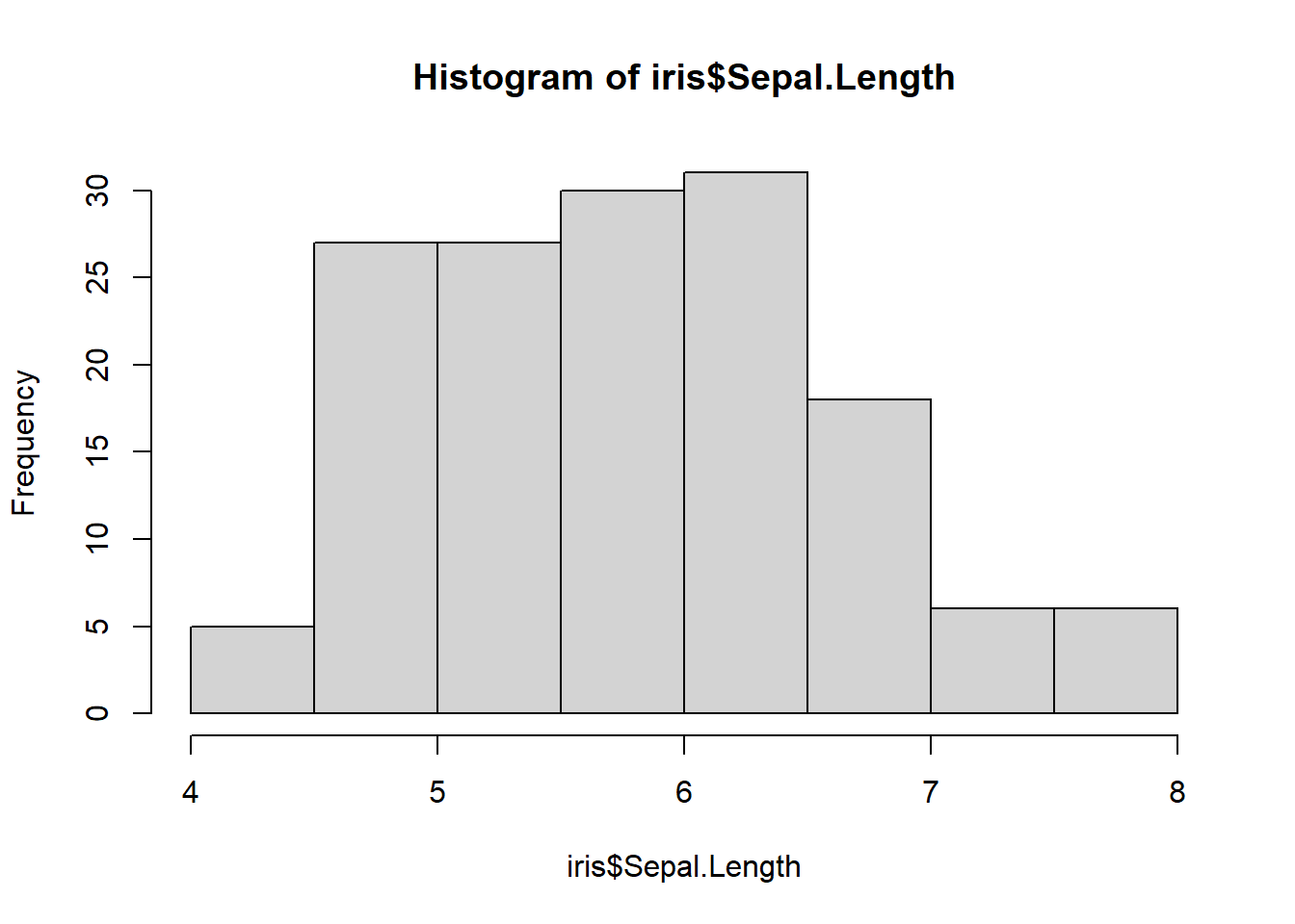
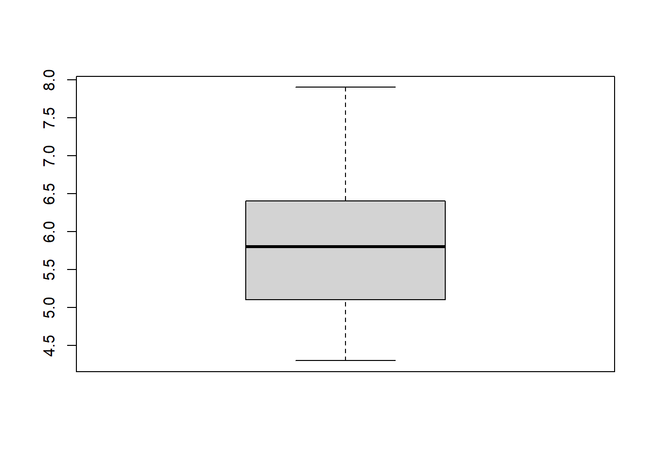
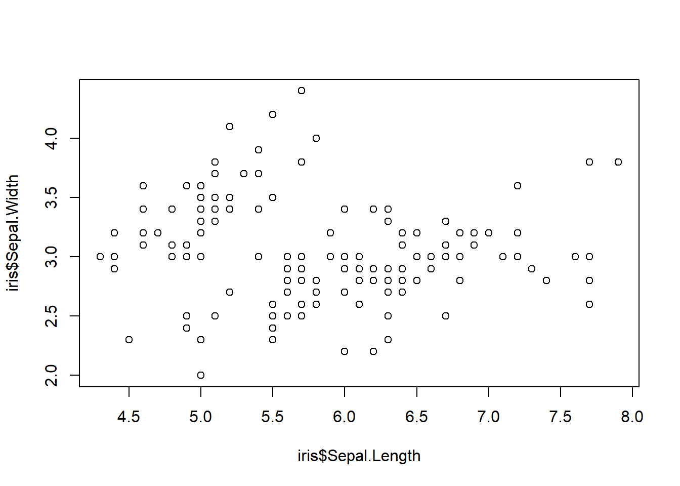
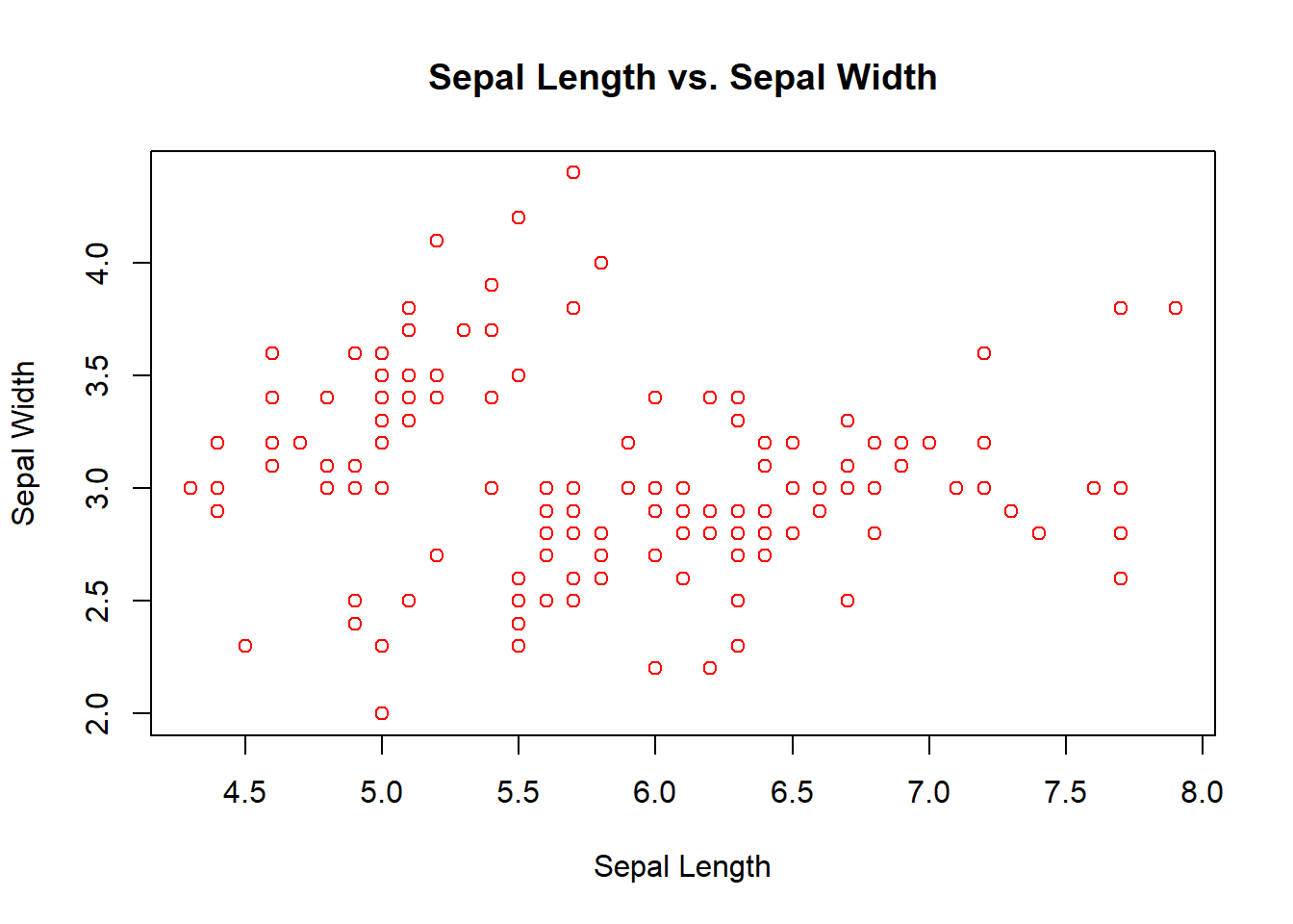
data(iris)
head(iris)
#>   Sepal.Length Sepal.Width Petal.Length Petal.Width Species
#> 1          5.1         3.5          1.4         0.2  setosa
#> 2          4.9         3.0          1.4         0.2  setosa
#> 3          4.7         3.2          1.3         0.2  setosa
#> 4          4.6         3.1          1.5         0.2  setosa
#> 5          5.0         3.6          1.4         0.2  setosa
#> 6          5.4         3.9          1.7         0.4  setosa
tail(iris)
#>     Sepal.Length Sepal.Width Petal.Length Petal.Width
#> 145          6.7         3.3          5.7         2.5
#> 146          6.7         3.0          5.2         2.3
#> 147          6.3         2.5          5.0         1.9
#> 148          6.5         3.0          5.2         2.0
#> 149          6.2         3.4          5.4         2.3
#> 150          5.9         3.0          5.1         1.8
#>       Species
#> 145 virginica
#> 146 virginica
#> 147 virginica
#> 148 virginica
#> 149 virginica
#> 150 virginica
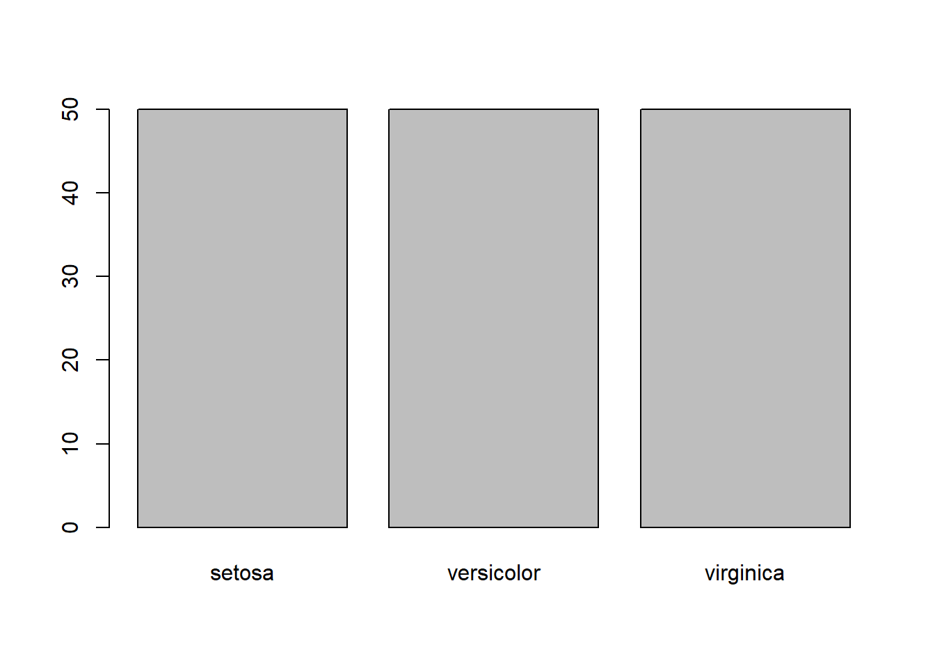
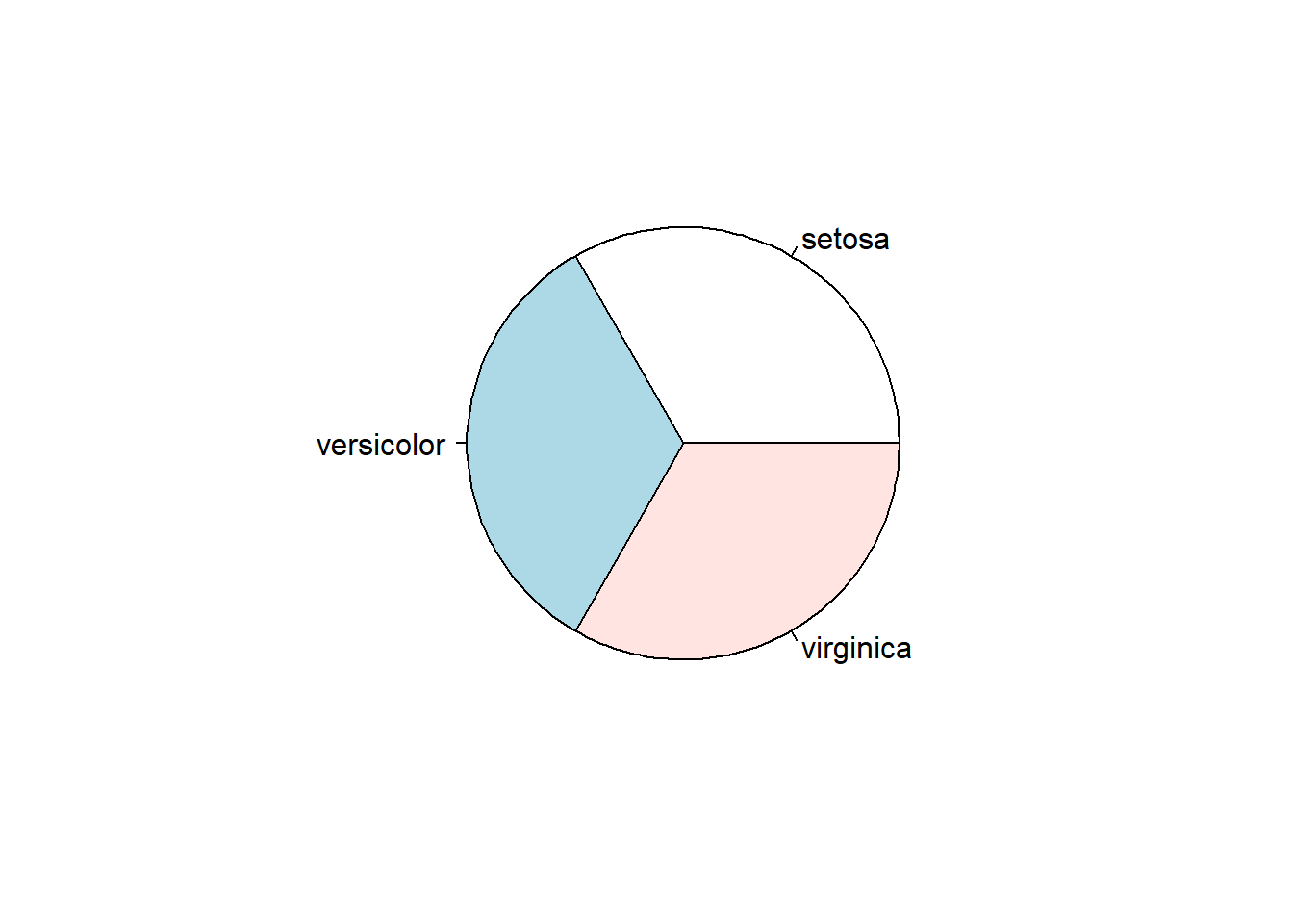
str(iris)
#> 'data.frame':    150 obs. of  5 variables:
#>  $ Sepal.Length: num  5.1 4.9 4.7 4.6 5 5.4 4.6 5 4.4 4.9 ...
#>  $ Sepal.Width : num  3.5 3 3.2 3.1 3.6 3.9 3.4 3.4 2.9 3.1 ...
#>  $ Petal.Length: num  1.4 1.4 1.3 1.5 1.4 1.7 1.4 1.5 1.4 1.5 ...
#>  $ Petal.Width : num  0.2 0.2 0.2 0.2 0.2 0.4 0.3 0.2 0.2 0.1 ...
#>  $ Species     : Factor w/ 3 levels "setosa","versicolor",..: 1 1 1 1 1 1 1 1 1 1 ...
1.3.1 R Package
# install.packages("readxl") - code to install R package
library(readxl)
#> Warning: package 'readxl' was built under R version 4.2.3
#install.packages("dplyr")
library(dplyr)
#> Warning: package 'dplyr' was built under R version 4.2.3
#>
#> Attaching package: 'dplyr'
#> The following objects are masked from 'package:stats':
#>
#>     filter, lag
#> The following objects are masked from 'package:base':
#>
#>     intersect, setdiff, setequal, union
1.3.2 Data Management With dplyr
head(iris)
#>   Sepal.Length Sepal.Width Petal.Length Petal.Width Species
#> 1          5.1         3.5          1.4         0.2  setosa
#> 2          4.9         3.0          1.4         0.2  setosa
#> 3          4.7         3.2          1.3         0.2  setosa
#> 4          4.6         3.1          1.5         0.2  setosa
#> 5          5.0         3.6          1.4         0.2  setosa
#> 6          5.4         3.9          1.7         0.4  setosa
irisbaru <- mutate(iris, sepal2 = Sepal.Length + Sepal.Width)
head(irisbaru)
#>   Sepal.Length Sepal.Width Petal.Length Petal.Width Species
#> 1          5.1         3.5          1.4         0.2  setosa
#> 2          4.9         3.0          1.4         0.2  setosa
#> 3          4.7         3.2          1.3         0.2  setosa
#> 4          4.6         3.1          1.5         0.2  setosa
#> 5          5.0         3.6          1.4         0.2  setosa
#> 6          5.4         3.9          1.7         0.4  setosa
#>   sepal2
#> 1    8.6
#> 2    7.9
#> 3    7.9
#> 4    7.7
#> 5    8.6
#> 6    9.3
irisetosa <- filter(iris, Species=="setosa")
head(irisetosa)
#>   Sepal.Length Sepal.Width Petal.Length Petal.Width Species
#> 1          5.1         3.5          1.4         0.2  setosa
#> 2          4.9         3.0          1.4         0.2  setosa
#> 3          4.7         3.2          1.3         0.2  setosa
#> 4          4.6         3.1          1.5         0.2  setosa
#> 5          5.0         3.6          1.4         0.2  setosa
#> 6          5.4         3.9          1.7         0.4  setosa
levels(iris$Species)
#> [1] "setosa"     "versicolor" "virginica"
irisversicolor <- filter(iris, Species=="setosa"& Petal.Length==1.3)
head(irisversicolor)
#>   Sepal.Length Sepal.Width Petal.Length Petal.Width Species
#> 1          4.7         3.2          1.3         0.2  setosa
#> 2          5.4         3.9          1.3         0.4  setosa
#> 3          5.5         3.5          1.3         0.2  setosa
#> 4          4.4         3.0          1.3         0.2  setosa
#> 5          5.0         3.5          1.3         0.3  setosa
#> 6          4.5         2.3          1.3         0.3  setosa
iris3 <- select(iris, Sepal.Length, Species)
head(iris3)
#>   Sepal.Length Species
#> 1          5.1  setosa
#> 2          4.9  setosa
#> 3          4.7  setosa
#> 4          4.6  setosa
#> 5          5.0  setosa
#> 6          5.4  setosa
iris4 <- arrange(iris, Petal.Width)
head(iris4)
#>   Sepal.Length Sepal.Width Petal.Length Petal.Width Species
#> 1          4.9         3.1          1.5         0.1  setosa
#> 2          4.8         3.0          1.4         0.1  setosa
#> 3          4.3         3.0          1.1         0.1  setosa
#> 4          5.2         4.1          1.5         0.1  setosa
#> 5          4.9         3.6          1.4         0.1  setosa
#> 6          5.1         3.5          1.4         0.2  setosa
iris4 <- arrange(iris, Species, desc(Petal.Width))
head(iris4)
#>   Sepal.Length Sepal.Width Petal.Length Petal.Width Species
#> 1          5.0         3.5          1.6         0.6  setosa
#> 2          5.1         3.3          1.7         0.5  setosa
#> 3          5.4         3.9          1.7         0.4  setosa
#> 4          5.7         4.4          1.5         0.4  setosa
#> 5          5.4         3.9          1.3         0.4  setosa
#> 6          5.1         3.7          1.5         0.4  setosa
names(iris4)[1] <- "length"
head(iris4)
#>   length Sepal.Width Petal.Length Petal.Width Species
#> 1    5.0         3.5          1.6         0.6  setosa
#> 2    5.1         3.3          1.7         0.5  setosa
#> 3    5.4         3.9          1.7         0.4  setosa
#> 4    5.7         4.4          1.5         0.4  setosa
#> 5    5.4         3.9          1.3         0.4  setosa
#> 6    5.1         3.7          1.5         0.4  setosa